CRE Certification Maths: Formulas, Worked Examples and a Study Plan

Most of the arithmetic on the ASQ CRE exam comes from a short list of formulas that keep returning in different clothes: exponential and Weibull reliability, series and parallel block arithmetic, availability, test sample sizes and chi-square confidence bounds. ASQ lets you carry a bound reference book into the room, so the skill being tested is choosing the right formula and keeping the numbers straight on a basic calculator. This guide works through each one with checked examples.

People who search for CRE certification usually want to know how hard the exam is. For an engineer who works in reliability every day the hard part is rarely the concepts. It is the arithmetic done cold, against a clock, with a calculator that cannot plot a distribution and a reference book that is only as useful as its index. Everything below is aimed at that gap.

Where does the arithmetic on the CRE exam actually sit?

The Body of Knowledge linked from ASQ's CRE page (checked October 2026) spreads the 150 scored questions over five areas: Reliability Fundamentals 29, Risk Management 25, Probability and Statistics for Reliability 35, Reliability Planning, Testing, and Modeling 35, and Lifecycle Reliability 26. Calculation is concentrated in the two 35-question areas, which together account for 70 of the 150 scored items, but it also turns up in smaller pockets elsewhere. The table lists the topics where you will be expected to compute something, with the highest cognitive level the CRE Body of Knowledge assigns to each.

Body of Knowledge topic	What you may have to compute	Highest level tested
I.B Basic reliability terminology	Failure rate, MTBF, MTTR, availability	Apply
III.A Probability distributions and functions	Binomial, Poisson, exponential, Weibull, normal, lognormal, chi-square and Student's t problems; CDF, PDF and hazard values	Analyze and Evaluate
III.A Sampling plans	Sample size or test time for a stated confidence	Apply
III.A SPC and capability studies	Cp, Cpk, Pp and Ppk, control chart limits	Apply
III.A Confidence and tolerance intervals	Interval estimates for Weibull, normal and lognormal data	Evaluate
IV.A and IV.B Test strategies, accelerated, qualification and demonstration testing	Zero-failure test size, acceleration factors, sequential and fixed-length test plans	Evaluate
IV.C Reliability block diagrams	Series, parallel, partial redundancy, K out of N, shared load	Evaluate
IV.C Failure models	Arrhenius, S-N curve and Coffin-Manson relationships	Analyze
V.A Stress-strength analysis and DOE	Probability of failure from two distributions; factorial designs with ANOVA	Analyze
V.C Maintainability	Preventive maintenance intervals, fault-isolation time, repair or replace time, crew hours	Apply

What the cognitive levels mean for the sums

The Body of Knowledge defines Apply as knowing when and how to use a formula, and Analyze and Evaluate as breaking a scenario into parts and judging between options. For arithmetic, that translates into two kinds of question. An Apply item hands you the numbers and expects you to run the right formula. An Analyze or Evaluate item buries the numbers in a scenario and makes you decide which model fits before you calculate anything. Practising only the first kind leaves a candidate fast at arithmetic and slow at setup, which is the wrong way round.

Risk Management and most of Reliability Fundamentals are mainly descriptive, so they need reading and recall rather than calculation. That is the reason the plan later in this guide gives its ten weeks to the maths and leaves the descriptive areas to ordinary revision.

Which core formulas does the CRE exam keep returning to?

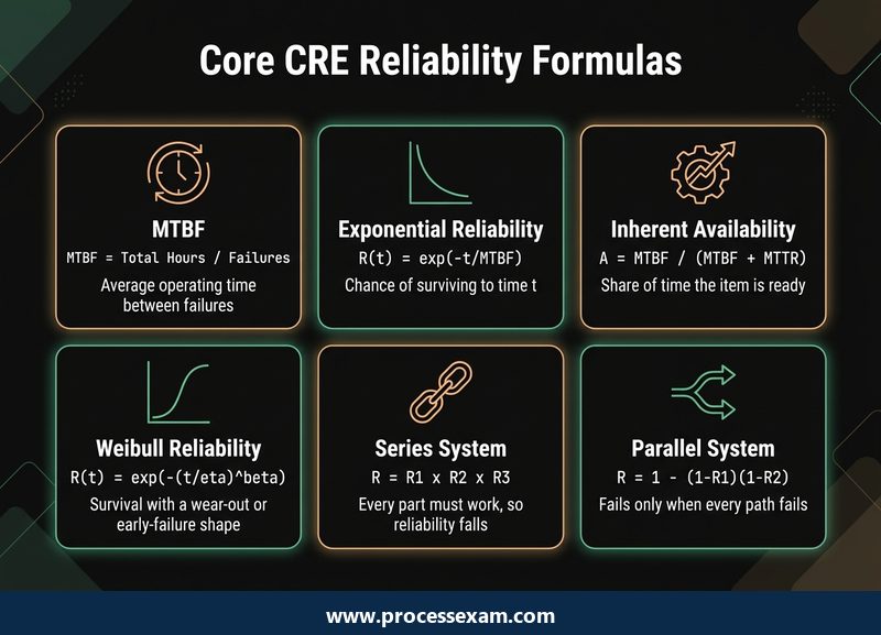
Six relationships cover a large share of the calculation items, and the card below puts them side by side. The examples that follow use round numbers so that you can repeat every step on a basic calculator and check that you land on the same answer.

Failure rate, MTBF and the exponential model

Twenty units run for 1,000 hours each, which is 20,000 unit-hours, and four of them fail. The failure rate is 4 / 20,000 = 0.0002 per hour, and the MTBF is the reciprocal, 20,000 / 4 = 5,000 hours. Under the exponential model the chance of surviving to time t is exp(-t / MTBF). For a 1,000-hour mission that is exp(-0.2) = 0.8187, so about 81.9 percent of units reach 1,000 hours without failing.

The classic trap sits at t equal to the MTBF itself. exp(-1) = 0.3679, so only about 36.8 percent of units survive to their own MTBF. Candidates who read MTBF as a guaranteed life choose the wrong answer on questions built around this. It also helps to remember what the model assumes: a constant failure rate. If the scenario describes wear-out or early-life failures, exponential is the wrong tool.

Repair time and availability

Suppose five corrective repairs took 2, 3, 5, 4 and 6 hours. MTTR is the mean, 20 / 5 = 4 hours. With the 5,000-hour MTBF above, inherent availability is MTBF / (MTBF + MTTR) = 5,000 / 5,004 = 0.9992. Inherent availability counts only active repair time, which is why it looks so good.

The Body of Knowledge also lists operational and achieved availability. Operational availability uses the mean time between maintenance and the mean downtime, which includes waiting for spares and people. If the same equipment sat idle for an average of 20 hours per stoppage and had no scheduled maintenance, operational availability would be 5,000 / 5,020 = 0.9960. The gap between 0.9992 and 0.9960 is the cost of logistics, and questions on this topic usually ask you to spot which definition the scenario needs.

The Weibull model and what its shape parameter says

Take a Weibull distribution with shape (beta) 2 and scale (eta) 1,000 hours. Reliability at 500 hours is exp(-(500 / 1,000) squared) = exp(-0.25) = 0.7788. The life by which 10 percent of units have failed, often called B10, comes from solving the reliability equation for t: t = eta x (-ln 0.90) to the power 1 / beta = 1,000 x 0.3246 = 324.6 hours.

The shape parameter tells you the failure pattern without any arithmetic. Below 1 the hazard falls with age, which suggests early-life failures; at exactly 1 the Weibull collapses to the exponential and eta equals the MTBF; above 1 it rises, which suggests wear-out. A subtle point worth rehearsing: for beta = 2 the mean life is eta x 0.8862 = 886 hours, not 1,000. Eta is the age by which 63.2 percent of units have failed, and it equals the mean only when beta is 1.

How do you work system reliability: series, parallel and K out of N?

Block diagram questions reward a fixed routine. Reduce the diagram from the inside out, collapse each parallel group into one equivalent block, then multiply along the series path. Three small cases show the pattern.

Series and parallel

Three blocks in series with reliabilities 0.98, 0.95 and 0.99 give 0.98 x 0.95 x 0.99 = 0.9217. Two blocks in parallel, each at 0.90, give 1 - (1 - 0.90) x (1 - 0.90) = 1 - 0.01 = 0.99. A mixed diagram has block A at 0.98, then a parallel pair of 0.90 blocks, then block C at 0.99. The pair collapses to 0.99, and the system is 0.98 x 0.99 x 0.99 = 0.9605.

Two sanity checks catch most slips. A series result can never exceed the weakest block, and a parallel result can never fall below the strongest. If your answer breaks either rule, the setup is wrong, whatever the calculator says.

K out of N

For two out of three identical blocks at 0.90, the system works if all three work or exactly two do: 0.90 cubed + 3 x 0.90 squared x 0.10 = 0.729 + 0.243 = 0.972. That sits between a single block at 0.90 and a three-way parallel arrangement at 0.999, which is what you would expect, because tolerating one failure is cheaper than tolerating two.

Bringing time into the diagram

Time-dependent items ask you to convert each block to a reliability at the mission time first, then combine. Two identical units in parallel, each with an MTBF of 5,000 hours, on a 1,000-hour mission: each unit has exp(-0.2) = 0.8187, so the pair gives 1 - (1 - 0.8187) squared = 1 - 0.0329 = 0.9671. Notice that the system MTBF is not simply 5,000 hours, because redundancy changes the shape of the system's failure pattern. Always combine reliabilities, never MTBFs, unless the question says the structure is simple enough for the shortcut.

Common-mode failure belongs in the same conversation. The independence assumed in every calculation above is exactly what a shared power supply or a shared environment destroys, and the Body of Knowledge lists common mode failure analysis separately for that reason.

How are test sizes, confidence bounds and acceleration factors worked out?

A zero-failure test sample size

To demonstrate a reliability R at confidence C by testing with no failures allowed, the number of units is n = ln(1 - C) / ln(R). For R = 0.90 at C = 0.90: ln(0.10) / ln(0.90) = -2.3026 / -0.1054 = 21.85, which you round up to 22 units. Raise the target to R = 0.95 at the same confidence and the answer becomes 2.3026 / 0.0513 = 44.9, so 45 units. Always round up, because rounding down quietly lowers the confidence you are claiming.

A lower confidence bound on MTBF

The point estimate from a test is only the centre of the story. Say a time-terminated test accumulates 10,000 unit-hours with 2 failures. The point estimate is 5,000 hours. A one-sided 90 percent lower bound for an exponential MTBF is 2T / chi-square, where T is the total test time and the chi-square value is the 90th percentile with 2r + 2 degrees of freedom, here 6. That percentile is 10.645, so the bound is 20,000 / 10.645 = 1,879 hours.

That is well under half the point estimate, which is the lesson of the exercise: few failures leave a wide interval. If the same 10,000 unit-hours had produced no failures, the chi-square value has 2 degrees of freedom, equals 4.605, and the bound becomes 20,000 / 4.605 = 4,343 hours. Be careful with the degrees of freedom. Time-terminated and failure-terminated tests use different counts, so check which version your reference gives and write it beside the formula in your index.

An Arrhenius acceleration factor

Arrhenius models temperature-driven failure. The acceleration factor is AF = exp[(Ea / k) x (1 / T-use - 1 / T-stress)], with temperatures in kelvin and k = 8.617 x 10 to the minus 5 electron-volts per kelvin. Take an activation energy of 0.7 eV, a use temperature of 55 degrees C (328.15 K) and a stress temperature of 105 degrees C (378.15 K). The bracket is 0.0030474 - 0.0026445 = 0.0004029, Ea / k is 8,123, their product is 3.273, and exp(3.273) = 26.4. A 1,000-hour stress test therefore stands in for roughly 26,400 hours at the use temperature, provided the same failure mechanism operates at both temperatures. The two classic errors are working in Celsius and forgetting to convert, and assuming that a higher stress is always valid.

Stress-strength interference

If strength is normal with mean 500 and standard deviation 40, and stress is normal with mean 400 and standard deviation 30, the item fails when stress exceeds strength. The margin has mean 500 - 400 = 100 and standard deviation the square root of (40 squared + 30 squared) = the square root of 2,500 = 50. That gives z = 100 / 50 = 2.00, and the normal table returns 0.9772, so the probability of failure is about 2.3 percent. The basic calculator cannot produce that table value, which is a good reason for the next section.

What does ASQ allow in the exam room, and how should a calculation reference be built?

ASQ's CRE page and its exam policies (checked October 2026) are explicit on three points. Every ASQ exam is open book, and you bring your own references. All reference material, including every form of notes, must be bound and stay bound: stitching, glue, ring binders, spiral binders, plastic snap binders and fasteners that pass through all the pages qualify, while loose or hand-stapled sheets do not. A test centre administrator inspects references before you enter. Sticky notes are permitted only as tabs and must already be attached when you arrive.

On calculators, the computer-based exam provides a basic scientific calculator on screen, and the test centre can lend a basic hand-held one on request. If you prefer your own, it must be silent, battery-operated and without programmable memory. ASQ names the Texas Instruments TI-89 and similar models as not allowed because they are programmable. Scratch paper and pencils are supplied at the centre.

What a basic calculator means for your book

A basic scientific calculator gives you logarithms, exponentials and powers, and nothing else. It has no normal distribution function, no chi-square percentile, no Weibull solver and no gamma function. Every value those need has to be looked up, so the tables are part of your preparation, not an afterthought. A reference built for calculation usually contains:

• A one-page formula index, arranged by Body of Knowledge topic, with the page of the longer treatment.
• One worked example per formula, written in your own hand with units, so you can compare structure at a glance.
• Normal, Student's t and chi-square tables, with the chi-square degrees-of-freedom rule for each test type written beside it.
• A small constants page: Boltzmann's constant in electron-volts per kelvin, the Celsius-to-kelvin conversion, and the gamma function values for common Weibull shape parameters.
• A wording guide that maps phrases such as "no failures allowed", "mean time to repair" and "at least one of two" to the formula they trigger.

Binding all of this is a design choice. A ring binder lets you add a page after a practice session reveals a gap, which a glued book does not, and the tabs can be attached at home before you travel. The CRE Handbook from ASQ Quality Press is the companion book the exam listing names, and many candidates treat it as the backbone and tab it heavily rather than carrying several books.

Calculator habits that save marks

Practise on the same type of calculator you will use, preferably the on-screen one, because its keypad behaves differently from a physical device. Enter exponents with explicit brackets, so exp(-t / MTBF) is not read as exp(-t) / MTBF. Carry at least five significant figures through a multi-step problem and round only at the end, since a rounded intermediate value can push an answer into the wrong option. Write each step on the scratch paper in the order you would explain it, because it is the quickest way to find an error when your answer matches no option.

How should the length of the paper shape your pace on calculation items?

The figures below are as listed for the CRE. Check them on ASQ's own page before applying, since fees and formats can change from one testing window to the next.

Exam detail	ASQ CRE
Exam	ASQ Certified Reliability Engineer (CRE)
Exam code	CRE
Number of questions	165
Duration	Total appointment time- 270 Exam Time - 258
Exam fee (USD)	ASQ MEMBERS - $450 NON-MEMBERS - $550 RETAKES - $350
Passing score	550/750

ASQ describes the computer-based paper as one part, with 150 questions scored and 15 unscored. You cannot tell which are the unscored ones. Spread 258 minutes over 165 questions and the average is about 94 seconds each. That average hides a wide spread: a definition or a terminology item takes seconds, while a confidence bound with a table lookup takes several times longer. The practical consequence is that your pace on the recall items funds your time on the calculations.

A two-pass approach to heavy items

On the first pass, answer everything you can in a single attempt and flag any question that needs more than one chain of calculation. Return to the flagged items with the time that remains. Because results are scaled to 750 points, with 550 needed to pass, a raw percentage is only an approximation of where you stand, so there is no virtue in sinking a quarter of an hour into one problem while easier marks wait.

Three ways the arithmetic goes wrong

Review of practice attempts tends to sort errors into three groups, and keeping a log under these headings tells you what to fix.

• Setup errors: the wrong model, such as exponential where the data show wear-out, or MTBF where MTTF applies to a non-repairable item.
• Lookup errors: the wrong table, the wrong degrees of freedom, or a one-sided value used where a two-sided one was needed.
• Keystroke errors: a missing bracket, a Celsius temperature in an Arrhenius sum, or rounding too early.

Setup errors are fixed by more scenario practice, lookup errors by a better index, and keystroke errors by the habits described above. They need different remedies, which is why a single overall practice score is a poor guide.

In what order should ten weeks of calculation practice run?

This plan covers only the calculation topics. It assumes you will read the descriptive areas in parallel or afterwards, and that you have a few evening sessions a week. Treat the week counts as a starting point and stretch them if statistics is not part of your daily work.

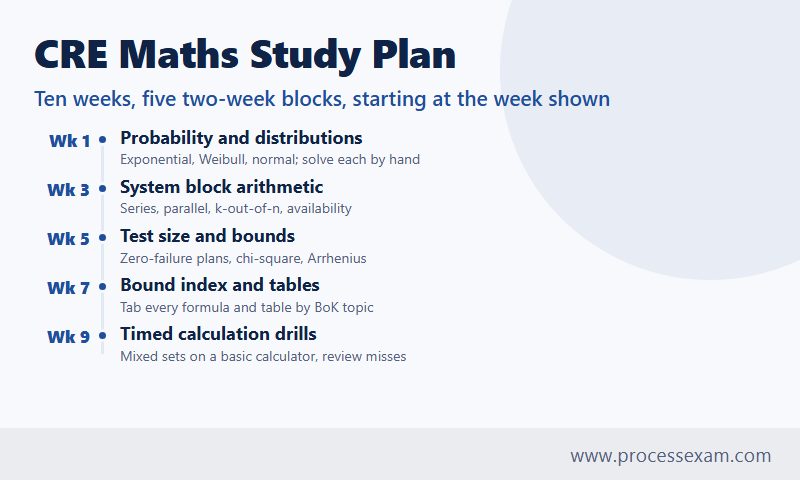
Weeks 1 and 2: distributions by hand

For each distribution the Body of Knowledge names, write down what it models, its parameters, and one problem you solve by hand. Do the exponential and Weibull examples above again with different numbers, then add a binomial and a Poisson case. Finish by reading a probability plot for a continuous distribution and judging whether the straight-line fit is believable, because goodness of fit is tested at the Analyze level.

Weeks 3 and 4: system and availability arithmetic

Draw ten block diagrams of your own, including a K out of N case and one with a shared load, and compute each by the reduce-then-multiply routine. Add three availability problems that force a choice between inherent, achieved and operational definitions. This is the block where sample questions help most, because you can attempt the style of item you will meet; ProcessExam's ASQ CRE sample questions are one place to try them.

Weeks 5 and 6: test sizes, bounds and accelerated testing

Work the zero-failure formula for five reliability and confidence pairs, then three chi-square bounds, one with zero failures. Repeat the Arrhenius calculation with an activation energy and temperatures of your own. End the block with a stress-strength problem, and record every table value you needed as a candidate for the index.

Weeks 7 and 8: the bound reference

Assemble the binder described earlier. Tab it by Body of Knowledge area, check every formula against the handbook rather than memory, and ask someone else to find three formulas in it while you watch. If they cannot find each one within a minute, the index needs work.

Weeks 9 and 10: mixed practice against the clock

Mix topics so that you have to choose the model, work on a basic calculator, and use only the bound reference. After each session sort your errors into the three groups above and revise the index accordingly. The CRE practice exam on ProcessExam follows the five areas of the Body of Knowledge, so a wrong answer points back to the block of this plan that needs reopening.

How to tell the plan is working

Three signs matter more than a score. Setup errors fall because you recognise wording patterns. The time you spend finding a table value drops to under a minute. And your hand calculations agree with the answer options to the third significant figure on the first attempt. When all three hold across two consecutive mixed sessions, the arithmetic is no longer what stands between you and a pass.

Frequently Asked Questions

Which parts of the ASQ CRE exam involve the most calculation?

Probability and Statistics for Reliability and Reliability Planning, Testing, and Modeling carry the most, at 35 scored questions each. Calculation also appears in terminology such as MTBF, MTTR and availability, in stress-strength analysis and in maintainability. Risk Management and most of Reliability Fundamentals are mainly descriptive, so they need recall rather than arithmetic.

Can you use a calculator on the CRE exam?

Yes. The computer-based exam includes a basic scientific calculator on screen, and the test centre can lend a basic hand-held one on request. A personal calculator must be silent, battery-powered and have no programmable memory. ASQ names the TI-89 and similar models as not allowed because they are programmable.

Is the CRE exam open book, and what counts as an allowed reference?

ASQ exams are open book and you supply the references. Everything, notes included, must be bound and remain bound: stitched, glued, or held by ring, spiral or snap binders. Hand-stapled loose sheets are refused. Sticky notes are accepted only as tabs fixed before you enter. A test centre administrator inspects references first.

How many questions are on the CRE exam and what is the passing score?

There are 165 questions on the computer-based exam, of which 150 are scored and 15 are unscored. Exam time is 258 minutes inside a 270-minute appointment. The passing score is 550 out of 750, a scaled result, so it is not the same as a percentage of questions answered correctly.

How long does it take to prepare the CRE calculation topics?

The plan in this guide allots ten weeks to the calculation topics: two weeks each for distributions, system arithmetic, test sizing and bounds, building a bound reference, and mixed timed practice. Engineers who use statistics daily may need less. Those who last studied it years ago should extend the first block.

Select ratingPoorOkayGoodGreatAwesome

Average: 5 (76 votes)