Statistics in Six Sigma: Which Tools Each Belt Needs

A bore that averages 10.1 mm, with a standard deviation of 0.12 mm and limits of 9.5 and 10.5 mm, has a Cpk of 1.11: (10.5 − 10.1) ÷ (3 × 0.12) = 0.40 ÷ 0.36. That single line uses a mean, a standard deviation and a capability index, which is about the arithmetic a Green Belt must handle. This guide shows how much statistics each belt needs, with the sums worked in full.

How much statistics does each Six Sigma belt actually need?

Less than the reputation suggests at the bottom, and more than most people expect at the top. Six Sigma is a way of replacing opinion with measurement, so every belt uses numbers, but the depth changes sharply. ASQ's three Bodies of Knowledge (all dated 2022) show the ladder clearly: the Yellow Belt describes data, the Green Belt judges whether a process meets its limits, and the Black Belt designs the study that proves a change worked.

The wording of each Body of Knowledge also carries a cognitive level in brackets, and that level tells you how the numbers will be tested. "Understand" means you can explain a term. "Apply" means you can use it on a new case. "Evaluate" means you can calculate it, interpret it and defend a decision based on it. The table below lists the statistical content only; the questions on leadership, deployment and Lean tools sit alongside it.

Belt	Statistics named in ASQ's Body of Knowledge	Level of testing
Yellow Belt	Mean, median, mode, range, variance and standard deviation; normal and binomial distributions; common versus special cause variation; correlation, regression and hypothesis-test vocabulary; X-bar and R charts	Apply for the basic statistics, Understand for everything else
Green Belt	Basic probability, the central limit theorem, normal, binomial, Poisson, chi square, t and F distributions; Cp, Cpk, Pp, Ppk and sigma shift; correlation and linear regression; paired t-test, F-test, ANOVA and chi square; X-R, X-s, ImR, median, p, np, c and u charts	Evaluate for descriptive statistics and capability, Analyze for the tests, Apply for charts
Black Belt	Everything above, plus sample-size calculation, confidence and prediction intervals, residual analysis, multivariate tools, goodness-of-fit tests, non-normal capability with Box-Cox transformation, rolled throughput yield, designed experiments, short-run and moving-average charts	Evaluate for most calculations, Apply for sample size and charts

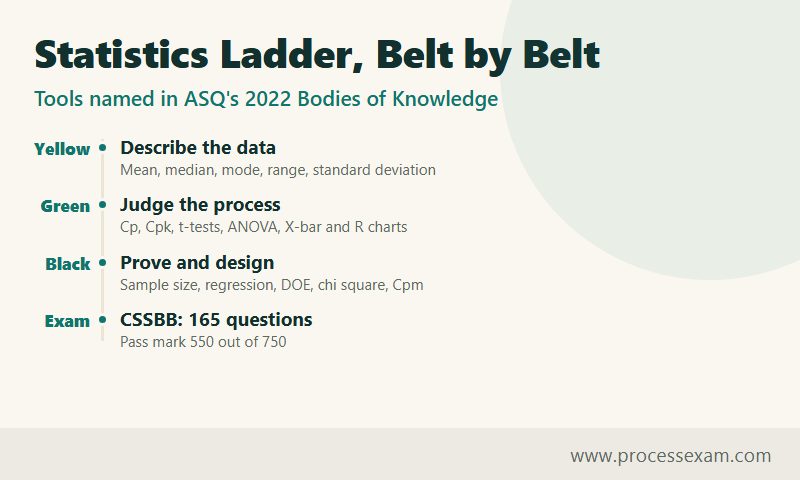
ASQ describes each credential on its own page: the Yellow Belt, Green Belt and Black Belt pages link to the full Body of Knowledge for each. The exams scale with the content. The computer-delivered Yellow Belt exam has 90 questions, the Green Belt 110 and the Black Belt 165, and all three are marked on a 750-point scale with 550 needed to pass.

The rest of this guide takes one calculation from each rung of the ladder, shows every step, and tells you which belt first meets it. If you can follow the arithmetic without software, you have the working statistics that a belt needs.

What do the mean, median, mode and standard deviation tell you about a process?

This is the Yellow Belt rung, and it is also the foundation for every later calculation. Take eight cycle times, in minutes, from one process: 12, 15, 11, 14, 13, 16, 12 and 15.

Centre: mean, median and mode

• Mean. Add the values: 12 + 15 + 11 + 14 + 13 + 16 + 12 + 15 = 108. Divide by 8 and the mean is 13.5 minutes.
• Median. Sort the values: 11, 12, 12, 13, 14, 15, 15, 16. With eight values the median is the average of the fourth and fifth, (13 + 14) ÷ 2 = 13.5 minutes.
• Mode. Both 12 and 15 appear twice, so the data set has two modes. A bimodal result is a hint that two different things are going on, perhaps two shifts or two machines, and it is worth a look before any further analysis.

Spread: range, variance and standard deviation

The range is the largest value minus the smallest, 16 − 11 = 5 minutes. It is quick, but it uses only two of the eight points. The standard deviation uses all of them:

1. Subtract the mean from each value: −1.5, +1.5, −2.5, +0.5, −0.5, +2.5, −1.5, +1.5.
2. Square each difference: 2.25, 2.25, 6.25, 0.25, 0.25, 6.25, 2.25, 2.25.
3. Add the squares: 22.0.
4. Divide by n − 1 = 7 to get the sample variance: 22 ÷ 7 = 3.14 square minutes.
5. Take the square root: the sample standard deviation is 1.77 minutes.

Dividing by n − 1 instead of n is the detail that people forget. The eight times are a sample, a statistic that estimates the unknown spread of the whole population, and a sample sits slightly closer to its own mean than to the true population mean. Dividing by 7 corrects that bias. If the eight values were the entire population, you would divide by 8 and the standard deviation would be 1.66 minutes. Both ASQ's Yellow Belt and Black Belt bodies of knowledge expect you to separate a population parameter from a sample statistic, so the difference is testable.

Notice what the mean alone would have hidden. A mean of 13.5 minutes sounds steady; a standard deviation of 1.77 minutes says that a typical order lands more than a minute and a half either side of it, and a customer promised "under 15" will be disappointed regularly. Every later tool, from capability to control charts, is a way of putting that spread to work.

How do Cp and Cpk turn spread into a verdict on the process?

This is the Green Belt rung, where "how much variation is there" becomes "is that good enough". Capability compares the width of the process with the width of the specification, using the standard deviation from the previous step.

Return to the opening example: a hole that must measure between 9.5 mm (the lower specification limit, LSL) and 10.5 mm (the upper limit, USL). The process mean is 10.1 mm and the standard deviation is 0.12 mm. Assume the data are roughly normal and the process is stable, which are the two conditions ASQ's Body of Knowledge asks you to verify before you quote a capability index.

Step by step

1. Cp, potential capability. Cp = (USL − LSL) ÷ (6 × standard deviation) = (10.5 − 9.5) ÷ (6 × 0.12) = 1.0 ÷ 0.72 = 1.39. If the process were perfectly centred, the spread would fit the tolerance almost one and a half times over.
2. Cpu, distance to the upper limit. (USL − mean) ÷ (3 × standard deviation) = (10.5 − 10.1) ÷ 0.36 = 0.40 ÷ 0.36 = 1.11.
3. Cpl, distance to the lower limit. (mean − LSL) ÷ (3 × standard deviation) = (10.1 − 9.5) ÷ 0.36 = 0.60 ÷ 0.36 = 1.67.
4. Cpk, actual capability. Cpk is the smaller of Cpu and Cpl, so Cpk = 1.11.

Cp (1.39) clears 1.33, a benchmark often used for a capable process, while Cpk (1.11) does not, and the gap between them is the story: the process is wide enough, but it is off-centre, drifting toward the upper limit. Moving the mean to 10.0 would lift Cpk to equal Cp, 1.39, with no change to the variation at all.

From Cpk to defects and sigma level

Cpk converts directly into a z-value: z = 3 × Cpk. The nearer limit is (10.5 − 10.1) ÷ 0.12 = 3.33 standard deviations away, which is a short-term sigma level of 3.33. The normal curve puts about 0.043% of parts beyond that limit, roughly 430 per million. The far limit sits (10.1 − 9.5) ÷ 0.12 = 5.0 standard deviations away and contributes less than one part per million, so the total is still about 430 parts per million.

Centre the same process at 10.0 mm and each limit is 0.5 ÷ 0.12 = 4.17 standard deviations away. The two tails then add up to about 31 parts per million, a fourteen-fold drop in defects from centring alone.

Short term versus long term

The figures above describe short-term capability. ASQ's Green and Black Belt bodies of knowledge both include the convention that a process drifts over the long run, and the customary allowance is a 1.5 standard-deviation shift. Applied to the 10.1 mm process, the nearer limit moves to 3.33 − 1.5 = 1.83 standard deviations away and the long-term defect rate climbs to roughly 33,400 per million, about 3.3%. The same machine looks very different depending on whether you quote the short-term or the long-term figure, which is why the Body of Knowledge asks candidates to say which one they are using. For a neutral background on the index itself, Wikipedia's article on the process capability index sets out Cp, Cpk, Pp and Ppk side by side.

How does a hypothesis test decide whether a change is real?

Yellow Belts meet the vocabulary of hypothesis testing; Green and Black Belts run the tests. The logic is the same every time: assume nothing has changed, measure how surprising your data would be if that were true, and reject the assumption only when the data are surprising enough.

Suppose the machine setting is supposed to produce a mean of 10.0 mm. After an adjustment, you measure nine parts. They average 10.12 mm with a sample standard deviation of 0.15 mm. Did the adjustment move the mean?

A one-sample t-test, step by step

1. State the hypotheses. The null hypothesis is that the true mean is still 10.0 mm. The alternative is that it differs from 10.0 mm. This is a two-sided test.
2. Choose the significance level. The conventional α = 0.05 means you accept a 5% risk of a type I error: declaring a change that is not there.
3. Calculate the standard error. 0.15 ÷ √9 = 0.15 ÷ 3 = 0.05 mm.
4. Calculate the test statistic. t = (10.12 − 10.0) ÷ 0.05 = 2.40.
5. Find the critical value. With n − 1 = 8 degrees of freedom, the two-sided 5% critical value of t is 2.306.
6. Decide. 2.40 is larger than 2.306, so reject the null hypothesis. The p-value is about 0.043, which is below 0.05.

The confidence interval agrees: 10.12 ± 2.306 × 0.05 = 10.12 ± 0.115, an interval from 10.005 to 10.235 mm. It just misses 10.0, which is exactly why the test rejects. Notice how marginal the result is. A p-value of 0.043 is not strong evidence; with one more unusual part the answer could flip.

Statistical versus practical significance

A 0.12 mm shift is statistically detectable, but the specification limits run from 9.5 to 10.5 mm. Whether it matters depends on the customer, not on the p-value. ASQ's Black Belt Body of Knowledge lists the contrast between statistical and practical significance as its own topic, and it is a favourite subject for scenario questions because the p-value alone never answers it.

How many parts should you have measured?

Black Belts are expected to calculate sample size, not merely run the test on whatever data exist. For a mean, the normal-approximation formula is n = (z for α/2 + z for β)² × σ² ÷ δ², where δ is the smallest shift you care about. To detect a 0.10 mm shift with a standard deviation of 0.15 mm, 5% significance and 80% power, use z = 1.96 and 0.84: n = (1.96 + 0.84)² × 0.15² ÷ 0.10² = 7.84 × 0.0225 ÷ 0.01 = 17.6, so 18 parts. A t-based calculation in software gives a slightly larger number, because the standard deviation is itself estimated, but the approximation is the right size for planning. The nine parts in the example were too few to detect a shift of 0.10 mm reliably, which is another reason the result above deserves caution.

How are control chart limits calculated from subgroups?

A capability study is a snapshot. A control chart is the film, and it answers a different question: is the process behaving the way it behaved before? Yellow Belts need to understand why X-bar and R charts are used, Green Belts build them, and Black Belts choose among a longer list of chart types.

Take a line that is sampled in subgroups of five parts. After 25 subgroups, the average of the subgroup means (the grand mean) is 10.02 mm and the average subgroup range, R-bar, is 0.30 mm. The constants for subgroups of five, taken from the standard table, are A2 = 0.577, D3 = 0 and D4 = 2.114.

The limits

• X-bar chart centre line: 10.02 mm.
• X-bar upper control limit: 10.02 + (0.577 × 0.30) = 10.02 + 0.173 = 10.193 mm.
• X-bar lower control limit: 10.02 − 0.173 = 9.847 mm.
• R chart centre line: 0.30 mm.
• R chart upper control limit: 2.114 × 0.30 = 0.634 mm.
• R chart lower control limit: 0 × 0.30 = 0, so there is no lower limit worth plotting.

The constant A2 is a shortcut for three standard errors. You can check it from first principles: the standard deviation estimated from ranges is R-bar ÷ d2 = 0.30 ÷ 2.326 = 0.129 mm, the standard deviation of a subgroup mean of five is 0.129 ÷ √5 = 0.058 mm, and three of those equal 0.173 mm, the same distance as above.

Control limits are not specification limits

This is the confusion that the Body of Knowledge keeps returning to, and it is worth stating plainly. Specification limits (9.5 and 10.5 mm in the earlier example) come from the customer and apply to individual parts. Control limits (9.847 and 10.193 mm here) come from the process and apply to subgroup averages. They have no mathematical relationship, which is why a process can be in control and still produce parts outside the specification, or be out of control while every part passes. Common-cause versus special-cause variation, the point behind the chart, is a Yellow Belt topic at the "Understand" level and an "Analyze" topic for Green and Black Belts, who must read run rules and patterns rather than just a single point beyond a limit.

Which statistics appear only at the Black Belt level?

The previous four sections cover what a Green Belt does with data and what a Black Belt must also be able to calculate. The Black Belt additions fall into three groups: relationships between variables, design of experiments, and yield and attribute measures.

Yield and defect arithmetic

The Black Belt Body of Knowledge asks for defects per unit, defects per million opportunities, first-pass yield and rolled throughput yield. Two short sums show the pattern.

• DPMO. A sample of 250 units, each with 4 opportunities for a defect, contains 18 defects. The defect rate per opportunity is 18 ÷ (250 × 4) = 18 ÷ 1,000 = 0.018, so the DPMO is 18,000.
• Rolled throughput yield. A process has three steps with first-pass yields of 98%, 97% and 95%. The chance that a unit passes all three first time is 0.98 × 0.97 × 0.95 = 0.903, so only 90.3% of units escape without rework even though no single step looks worse than 95%.

Modelling and experiments

Correlation, regression, analysis of variance, chi-square tests and designed experiments take the same logic as the t-test above and extend it to several variables or several groups at once. The Black Belt Body of Knowledge asks candidates to calculate and interpret a correlation coefficient and its confidence interval, to test regression statistics, to analyse residuals and to select, calculate and interpret ANOVA. In Improve it expects full factorial and fractional factorial experiments, with confounding and resolution as vocabulary. Non-normal data bring Box-Cox transformation into the capability study, and attribute data use their own capability and sigma-level calculations.

The weight of these topics inside the CSSBB exam is considerable. ASQ's 2022 Body of Knowledge lists Measure at 25 questions, Analyze at 22, Improve at 21 and Control at 17, and each of those sections carries statistics. The first three sections, on deployment, process management and teams, add 39 more between them.

CSSBB exam detail	Figure
Exam code	CSSBB
Vendor	ASQ
Questions	165 (ASQ marks 150 as scored and 15 as unscored)
Duration	270 minutes total appointment time, 258 minutes exam time
Exam fee	ASQ members $485, non-members $585, retakes $385
Passing score	550/750
Open book	Yes, with bound reference material

For the full structure of that exam, ASQ's Black Belt page is the authoritative source, and this site's CSSBB exam syllabus page lists the topic areas for revision.

Which traps catch people who compute these figures by hand?

Almost every wrong answer in a statistics question comes from one of a short list of slips. Each of them appears in the worked examples above, which makes them easy to practise on.

• Dividing by n instead of n − 1. For the eight cycle times, 1.66 and 1.77 are both "standard deviations", and only one is right for a sample. The question wording tells you which.
• Quoting Cp when Cpk was asked, or the reverse. Cp ignores where the mean sits. A process can have a Cp of 1.39 and still be producing defects, because the mean has drifted toward a limit.
• Calculating a capability index on an unstable process. Cpk assumes the process is stable and roughly normal. If the control chart shows special causes, the index describes a moment, not the process, and the Body of Knowledge expects you to check stability first.
• Mixing up control limits and specification limits. The first belong to the process and the second to the customer. A control limit tells you nothing about whether a part is acceptable.
• Reading a p-value as the chance the null hypothesis is true. A p-value of 0.043 means that data this extreme would appear about 4.3% of the time if the mean really were 10.0. It does not mean there is a 4.3% chance nothing changed.
• Treating "not rejected" as "proved equal". A test with nine parts that fails to reject has simply failed to find a difference; with too few parts it never had much power to find one.
• Forgetting the units after squaring. Variance is in square minutes or square millimetres. Only the standard deviation returns to the original unit.

A useful check is to ask what each answer should look like before you calculate. A standard deviation of 15 minutes for data that lie between 11 and 16 is impossible, and noticing that takes ten seconds.

Do you need statistical software, or is a calculator enough?

For learning, a calculator is enough, and doing the arithmetic once by hand is what makes the software output meaningful. In practice, Black Belts use software for regression, ANOVA and designed experiments, because those calculations involve matrices and many observations. The skill that the credential tests is not the keystrokes but the judgement around them: choosing the right test, checking its assumptions and explaining the result to someone who does not know statistics.

The exam reflects that. According to ASQ, the CSSBB is open book, and the computer-based exam provides an on-screen basic scientific calculator, with a basic hand-held model available on request. Personal calculators must be silent and battery-operated, and programmable models are not allowed. That puts the sums above, the standard deviation, Cpk, a t-statistic, control limits from a table of constants, squarely in the range of what you must be able to do quickly with a basic scientific calculator and your own bound notes.

A practice routine that uses the examples

1. Redo each worked example once without looking at the steps, then check every intermediate figure rather than just the answer.
2. Change one input and predict the effect before you calculate. What happens to Cpk if the standard deviation falls to 0.10? (Cpu becomes 0.40 ÷ 0.30 = 1.33.) What happens to the t-statistic if the sample has 16 parts instead of nine? (The standard error shrinks to 0.0375 and t rises to 3.2.)
3. Write the constants you will need, such as A2, D3, D4 and d2 for subgroups of two to ten, on one tabbed page of your reference material.
4. Finish with timed questions, because an exam of this length rewards a steady pace as much as accuracy.

When you want to see whether these calculations hold up under exam conditions, the CSSBB practice exam gives you full-length scenario questions on the same statistical tools to try against the clock.

Frequently Asked Questions

How much statistics do you need for Six Sigma?

It depends on the belt. A Yellow Belt needs the mean, median, mode, range and standard deviation, plus an understanding of control charts. A Green Belt adds capability indices, t-tests and ANOVA. A Black Belt also plans sample sizes, builds regression models and designs experiments, using software for the heavy calculations.

What is the statistical meaning of Six Sigma?

Statistically, six sigma means the nearest specification limit sits six standard deviations from the process mean. With the customary 1.5 standard-deviation long-term shift allowed, that corresponds to 3.4 defects per million opportunities. Many real processes run at far lower sigma levels, and the metric is mainly a way of comparing them.

What is the difference between Cp and Cpk?

Cp compares the width of the specification with the width of the process spread and ignores where the mean sits. Cpk uses the distance from the mean to the nearer specification limit, so it falls when the process is off-centre. Cpk can never exceed Cp, and the two are equal only for a centred process.

What statistics are on the CSSBB exam?

ASQ's 2022 Body of Knowledge covers descriptive statistics, probability distributions, process capability, correlation and regression, hypothesis tests, ANOVA, sample size, designed experiments and control charts. Statistical content runs through the Measure, Analyze, Improve and Control sections, which together carry most of the scored questions.

Can you use a calculator in the CSSBB exam?

Yes. ASQ provides an on-screen basic scientific calculator in the computer-based exam and will supply a basic hand-held model on request. Candidates may bring a silent, battery-operated calculator without programmable memory. Programmable models such as the TI-89 are not permitted, so practise the sums on a basic model.

Select ratingPoorOkayGoodGreatAwesome

Rating: 4.9 / 5 (85 votes)