CSSGB Calculations: Cp, Cpk, Control Limits and DPMO Worked Out

A machine turns out shafts specified at 10.00 mm plus or minus 0.30, and the spread is tight: a standard deviation of 0.04 mm. Cp comes out at 2.50, which looks superb. Then the mean turns out to sit at 10.20 mm, and Cpk falls to 0.83, about six shafts in every thousand over the upper limit. That gap between two capability numbers is the kind of arithmetic the ASQ Certified Six Sigma Green Belt (CSSGB) exam rewards.

Candidates searching for CSSGB questions or CSSGB exam questions usually expect definitions. A good share of the items ask for a number instead, and the number is rarely hard: one or two steps, a formula you have seen, a table you can carry in. What goes wrong is the set-up, a wrong formula or a slipped digit that lands on a plausible-looking option. For anyone aiming at the ASQ Green Belt certification, this guide covers the topics that need arithmetic, works one illustration of each, and shows how to handle them quickly under ASQ's calculator and reference rules. Every figure in the worked examples is invented here to show the method; none comes from an exam.

Which CSSGB topics need arithmetic, and how hard is it?

ASQ's 2022 Body of Knowledge tells you where the numbers sit. Its verbs are the clue: wherever a topic says calculate, the exam can hand you data and ask for a result. Reading the PDF for that one word turns the syllabus into a short list of computing jobs, and it is the quickest way to decide how much of your study time belongs to the calculator rather than to reading.

Topic area	What you may be asked to compute	Where to start
Process capability	Cp, Cpk, Pp and Ppk from limits, a mean and a standard deviation	Distance from the mean to the nearer limit, divided by three standard deviations
Control charts	Centre line and limits for X-bar and R, individuals, p, np, c and u charts	Pick the chart from the data type, then the constant or the square root
Process performance	Defects per unit, defects per million opportunities, rolled throughput yield, sigma level	Count defects against units and opportunities, then convert with a table
Hypothesis testing	A test statistic, a decision against a critical value, the sample size for a target margin	Match the test to the data, then compare statistic with critical value
Risk and cost	A risk priority number from failure mode ratings, cost of poor quality	Multiply severity, occurrence and detection, or add the cost categories

Notice what is missing: no derivations, no proofs, no matrix algebra. Even the biggest items are a short chain of operations on a basic scientific calculator. The difficulty is choosing the right chain under time pressure, which is a habit you build by repetition rather than by reading, and the option lists are written to punish a wrong chain with an answer that looks close. A risk priority number is the gentlest example: severity 7, occurrence 5 and detection 4 multiply to 140, and the only trap is adding instead of multiplying.

Why the numbers deserve study time

The pass mark on the CSSGB is 550 out of 750 on ASQ's scaled score, so you can miss a fair share of items and still pass. That makes arithmetic a place to bank marks, because a calculation has one right answer while a definition question often has two arguable ones. Candidates who skip the numerical items to save time for the wording-heavy ones often find afterwards that the numerical ones were the cheaper marks.

The calculation topics also sit at the heart of a Green Belt's day job. A capability study, a control chart and a defect rate are what you will be asked to produce in a real project, so time spent here pays twice: once on the exam and once at work. That is also why the exam treats them at the Analyze level, where you must choose and apply the method, not merely recognise its name.

How do Cp and Cpk tell different stories about the same process?

Cp compares the width of the specification with the width of the process: the upper limit minus the lower limit, divided by six standard deviations. It ignores where the process sits. Cpk adds the position: it takes the distance from the mean to the nearer limit and divides by three standard deviations. When the process is dead centre the two are equal; when it drifts, Cpk falls below Cp and never exceeds it.

Worked illustration: the shaft

Limits are 9.70 and 10.30, so the spread of the specification is 0.60. The standard deviation is 0.04, so six standard deviations are 0.24.

1. Cp = 0.60 / 0.24 = 2.50.
2. The mean is 10.20. Distance to the upper limit: 10.30 minus 10.20 = 0.10. Distance to the lower limit: 10.20 minus 9.70 = 0.50.
3. The nearer side is the upper one, so Cpk = 0.10 / (3 x 0.04) = 0.10 / 0.12 = 0.83.

The upper limit is only 0.10 / 0.04 = 2.5 standard deviations from the mean, so the share beyond it on a normal curve is about 0.62 per cent, roughly 6,200 parts per million. Move the mean back to 10.02 and Cpk becomes 1.56 with the same spread, because both limits are now far away. That is the story of the opening paragraph: Cp measures what the process could do if centred, Cpk what it does.

A shortcut worth carrying: Cpk is a distance in sigmas

Three times Cpk is the number of standard deviations between the mean and the nearer limit. That gives you a quick conversion to a defect rate, and it lets you check an answer without a formula. The tail figures below assume a normal curve and count only the nearer side.

Cpk	Sigmas to nearer limit	Parts per million beyond it
0.83 (the shaft)	2.5	about 6,200
1.00	3.0	about 1,350
1.33	4.0	about 32
1.67	5.0	about 0.29

Pp and Ppk use the same formulas, but with the standard deviation of all the data rather than the within-subgroup estimate. A question that gives you two standard deviations is testing whether you know which one belongs to which index. If the overall spread on the shaft is 0.05, Pp is 0.60 / 0.30 = 2.00 while Cp stays at 2.50, and the difference warns that the process moves between subgroups.

The sigma-level questions come with a convention you need to recognise: the long-run mean is assumed to drift by 1.5 standard deviations relative to the short-term data. That is why a process with a 6 sigma short-term distance is quoted at 3.4 defects per million, not at the far smaller figure a centred normal curve would give. When a question mentions short-term and long-term data together, it is asking about that shift.

How do you set control chart limits without deriving anything?

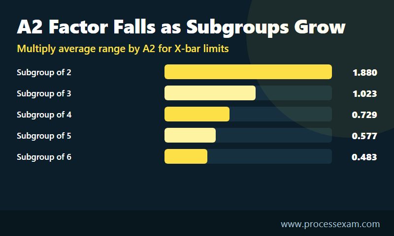
Control limits are not specification limits. They are three standard deviations either side of the centre line for the statistic you plot, and they describe what the process does, not what the customer wants. The exam tests both the arithmetic and the chart choice: measured data points to X-bar and R, X-bar and s, or individuals; counts point to p, np, c or u. Once the chart is chosen, the arithmetic is one multiplication from a constant.

Subgroup size	A2 (X-bar limits from R-bar)	D3 (lower R limit)	D4 (upper R limit)
2	1.880	0	3.267
3	1.023	0	2.574
4	0.729	0	2.282
5	0.577	0	2.114
6	0.483	0	2.004

Worked illustration: X-bar and R with subgroups of five

Suppose the grand average of the subgroup means is 50.2 and the average range is 3.1.

1. X-bar upper limit = 50.2 + 0.577 x 3.1 = 50.2 + 1.79 = 51.99.
2. X-bar lower limit = 50.2 - 1.79 = 48.41.
3. R upper limit = 2.114 x 3.1 = 6.55. The lower limit is 0 x 3.1 = 0, so the chart has no lower range limit.

If a question wants the process standard deviation from the same data, divide the average range by the constant d2, which is 2.326 for subgroups of five: 3.1 / 2.326 = 1.33. Using the average range directly as a standard deviation is a classic wrong option. Notice, too, that the constants shrink as subgroups grow: bigger subgroups average out more noise, so the limits on the means pull in.

Worked illustration: a p chart with a lower limit that goes negative

Take an average fraction defective of 0.04 and a constant sample of 200. The standard error is the square root of 0.04 x 0.96 / 200, which is 0.0139. The upper limit is 0.04 + 3 x 0.0139 = 0.082. The lower limit works out at 0.04 - 0.0416 = -0.0016, and a fraction cannot be negative, so the limit is set at zero. A question that offers a negative lower limit as an option is testing exactly this.

The reading rules that follow the arithmetic are also tested: a point beyond a limit, a long run on one side of the centre line, a steady trend. Know them as tests of whether the process changed, not as a calculation, and remember that a chart showing such signals means the process is not yet stable enough for a capability index to mean much.

How do you get from a defect count to DPMO and a sigma level?

Process performance questions share one vocabulary, and the arithmetic is a ladder: defects per unit, defects per opportunity, defects per million opportunities, then a conversion to yield and sigma level. Climbing it in order stops you mixing the denominators, which is the commonest way to land on an option that is exactly a factor out.

Worked illustration: a billing run

A team inspects 500 invoices, each with 8 fields that can be wrong, and finds 42 errors in total.

1. Defects per unit = 42 / 500 = 0.084.
2. Opportunities = 500 x 8 = 4,000, so defects per opportunity = 42 / 4,000 = 0.0105.
3. DPMO = 0.0105 x 1,000,000 = 10,500.
4. Yield per opportunity = 1 - 0.0105 = 98.95 per cent. A normal table gives a z value of about 2.31 for that yield.
5. Adding the 1.5 shift convention gives a sigma level of about 3.81.

Forgetting the opportunities and dividing 42 by 500 gives 84,000, which is eight times too large. A question built that way will list 84,000 among the options.

Rolled throughput yield multiplies, it does not average

Three process steps yield 98, 95 and 99 per cent. Rolled throughput yield is the product: 0.98 x 0.95 x 0.99 = 0.9217, or 92.2 per cent. The average of the three, 97.3 per cent, is the tempting wrong option, and the sanity check is quick: the rolled figure can never exceed the weakest step. Where a question gives defects per unit instead, yield is approximately e raised to the minus DPU, so the 0.084 above gives about 0.919.

A word on the table you will need: a normal table in your bound reference saves you from inverting the curve in your head. A basic scientific calculator will not convert a yield to a z value for you, so questions of this kind either supply the table value or expect you to read it from the reference you carry. Mark the page, and note beside it whether your table shows the area to the left of z or the tail beyond it, because the two read differently.

What do hypothesis-test and sample-size questions expect you to compute?

Here the exam splits its weight. Some items give you a test statistic and ask for the decision; others ask which test fits the data; a smaller group wants you to build the statistic yourself. The statistics are plain: a difference divided by its standard error.

Worked illustration: a one-sample t test

A filling line is supposed to average 50.0. A sample of 16 gives a mean of 52.4 and a standard deviation of 4.0.

1. Standard error = 4.0 / the square root of 16 = 1.0.
2. t = (52.4 - 50.0) / 1.0 = 2.40, with 15 degrees of freedom.
3. The two-sided critical value at the 5 per cent level and 15 degrees of freedom is 2.131, and 2.40 is beyond it, so you reject the claim that the mean is 50.0.

Rejecting is a statement about evidence, not about size. Statistical significance and practical significance are separate ideas in the syllabus, and a question may give you a result that is significant but too small to matter to the customer.

Worked illustration: how many samples?

To estimate a mean to within plus or minus 1.0 at 95 per cent confidence, with a standard deviation of about 4.0, use n = (1.96 x 4.0 / 1.0) squared = 61.5, and round up to 62. The rounding direction is the trap: 61 would leave the margin slightly too wide, so sample-size answers always go up. For a proportion with no prior estimate, use 0.5 for the unknown fraction: 1.96 squared x 0.25 / 0.05 squared = 384.2, so 385 for a margin of five percentage points.

Type I error is rejecting a true claim, set by the significance level; type II is failing to reject a false one, and power is one minus that. Knowing which is which is worth more marks than any arithmetic here, because many options are just different wordings of the same two ideas. Across the named tests (paired t, F, analysis of variance and chi-square among them), learn what kind of data each one expects before you learn its formula.

How do ASQ's calculator and reference rules change the way you work a number?

ASQ's Six Sigma Green Belt page sets the rules, and they shape the technique. Every ASQ exam is open book. The computer-based exam shows a basic scientific calculator on screen, the test centre administrator will hand you a hand-held basic calculator on request, and you may bring your own as long as it is silent, battery-powered and has no programmable memory. ASQ lists graphing, storing user text and function keys as signs of a programmable machine, and names the Texas Instruments TI-89 as an example that is not allowed. The test centre provides scratch paper and pencils.

Reference material must be bound and stay bound: stitched, glued or held in a binder by fasteners that go through the pages. Post-it notes are permitted as tabs only, attached before you enter the test centre, and the administrator inspects your references first. Read the policy as ASQ prints it before you buy a binder, since a spiral or ring binder is accepted but a hand-stapled bundle that is not held in a cover is not.

Exam fact	Figure
Exam code and vendor	CSSGB, ASQ Certified Six Sigma Green Belt
Questions	110
Exam time	258 minutes (270 minutes total appointment time)
Passing score	550/750
Price	$383 for ASQ members, $483 for non-members, $283 for retakes

Turn the rules into a routine

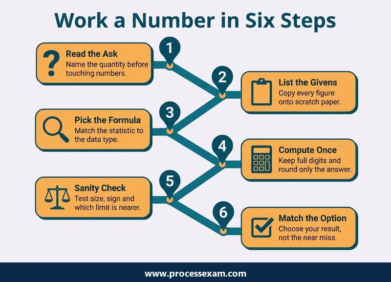
Four habits make the rules work for you. First, practise on a basic scientific calculator with the same key sequence you will use on the day, including how it handles brackets, powers and square roots. Second, write the formula and the givens on scratch paper before touching a key; a mistyped number is easy to find when it is written down and nearly impossible to find when it is not. Third, keep full digits until the final step and round only the answer, since early rounding is how a standard error of 0.0139 becomes a neighbouring option. Fourth, put a worked example next to each formula in your own bound sheet, so that a looked-up formula comes with its own reminder of how to use it.

Time is the other constraint. With 110 questions and a little over four hours of exam time, a calculation item can afford a few minutes, but only if the definition items are answered quickly. Decide up front that a numerical question gets a clean set-up, one computation and one sanity check, and no more; flag it and move on if it does not settle.

Four sanity checks that take seconds

• Cpk can never exceed Cp, so an answer that does is wrong.
• A rolled yield can never exceed its weakest step.
• An upper control limit sits above the centre line and a lower one below it, and a fraction or count limit below zero is set to zero.
• A sample size is a whole number, always rounded up.

Which wrong options are built from a calculation slip?

Multiple-choice writers build distractors from the mistakes real candidates make, so a wrong option is often the result of one specific slip. Recognising the slip tells you the question's trap and lets you check your own number against a list.

Slip	What it produces in our examples	Check
Using the farther limit for Cpk	0.50 / 0.12 = 4.17 instead of 0.83	Cpk comes from the nearer limit and cannot exceed Cp
Using six sigmas in Cpk	0.10 / 0.24 = 0.42 instead of 0.83	Cp uses six, Cpk uses three
Treating the average range as a standard deviation	A spread of 3.1 instead of 1.33	Divide the range by d2
Leaving opportunities out of DPMO	84,000 instead of 10,500	Divide by units times opportunities
Averaging step yields	97.3 per cent instead of 92.2	Multiply them; the result sits below the weakest step
Rounding a sample size down	61 instead of 62	Always round up
Mixing control and specification limits	A plotted point judged against 9.70 and 10.30	Control limits come from data, specification limits from the customer

The two slips that cost the most are conceptual, not arithmetical: choosing the wrong chart for the data type, and reading a capability index from a process that is not in control. A capability index describes a stable process, so a question that shows a chart with points beyond the limits is telling you to fix stability first.

How should you drill the arithmetic in the weeks before the exam?

Treat the calculation topics like a language you speak aloud: short daily sessions beat one long weekend. Each day, take one formula from the tables above, change every figure in the worked example, and recompute it from scratch on your exam calculator, then write down the sanity check that would have caught a slip. Rotate through capability, charts, DPMO, tests and sample size over a week, then repeat with different numbers.

Pair the drills with the syllabus structure rather than with a random set of formulas. A short pass through the CSSGB sample questions shows how ASQ-style items phrase a calculation, which tells you which of your formulas to tab. Build the formula sheet from your own failed attempts, not from a textbook index: a formula you have already got wrong once belongs on it.

Run the numerical items of the CSSGB practice exam against your formula sheet, and sort the wrong answers by cause: set-up, arithmetic or reading of the question, because each of the three needs a different remedy.

Finally, remember what the arithmetic is for. A Green Belt who can compute Cpk but cannot say what to do about a 0.83 has learned the formula without the purpose. The exam's calculation items and its scenario items are two views of the same skill, which is deciding from data whether a process is capable, stable and worth changing, and the opening shaft is a fair model of it: two numbers, one story, and a decision about which to trust.

Frequently Asked Questions

Is the CSSGB exam heavy on maths?

No. The arithmetic is modest: capability indices, control chart limits, DPMO and sigma level, a test statistic and a sample size, each a short chain on a basic scientific calculator. The risk lies in choosing the wrong formula or rounding early, so practise the set-up as much as the sums.

Can you use a calculator on the ASQ Green Belt exam?

Yes. The computer exam shows a basic scientific calculator on screen, and the test centre administrator can hand you a hand-held basic one on request. You may bring your own if it is silent, battery-powered and not programmable. ASQ names the TI-89 as not allowed.

What do CSSGB exam questions look like?

They are multiple choice, 110 in the exam, and many test a topic at the Analyze level with a short scenario or a set of figures. A number-based item gives you data and expects a result that matches one option, so the wrong options are usually common slips.

What score passes the CSSGB certification, and what does it cost?

ASQ sets the passing score at 550 out of 750. The exam costs $383 for ASQ members and $483 for non-members, and a retake costs $283. The computer exam allows 258 minutes of exam time inside a 270 minute appointment.

Which formulas should you put in your bound reference for the CSSGB?

Carry the capability formulas, the control chart constants A2, D3, D4 and d2, the DPMO and yield steps, the t statistic and the sample-size formulas, plus a normal table. Add a worked example beside each. ASQ requires references to be bound, with Post-it notes allowed only as tabs.

Select ratingPoorOkayGoodGreatAwesome

Average: 4.9 (78 votes)